Example 1 — 2D Grey Participating Medium

Last updated

30 September 2026

This example solves radiative equilibrium in a 1 × 1 m square enclosure filled with an absorbing gas (absorption coefficient κ = 1 m⁻¹, no scattering: σₛ = 0 m⁻¹). The bottom wall is held at 1000 K and all other walls are at 0 K; all surfaces are black (ε = 1). The gas temperature field is found by solving the GERT system after computing exchange factors by ray tracing.

Step 1: Define the geometry and mesh

using RayTraceHeatTransfer
using GeometryBasics, StaticArrays

function build_mesh(Ndim)                          # define a mesh builder function
    vertices = SVector(
        Point2(0.0, 0.0),
        Point2(1.0, 0.0),
        Point2(1.0, 1.0),
        Point2(0.0, 1.0)
    )
    solidWalls = SVector(true, true, true, true)   # all walls impenetrable by radiation

    face = PolyVolume2D{Float64}(vertices, solidWalls, 1, 1.0, 0.0)   # κ = 1, σₛ = 0 for the gas volume

    face.T_in_w  = [1000.0, 0.0, 0.0, 0.0]        # bottom hot, rest cold
    face.epsilon = [1.0, 1.0, 1.0, 1.0]            # black walls
    face.T_in_g  = -1.0                            # unknown (solve for this)
    face.q_in_g  = 0.0                             # radiative equilibrium

    mesh = RayTracingDomain2D([face], [(Ndim, Ndim)]; verbose = false)   # mesh the domain
    return mesh
end
Ndim  = 11                                         # 11 × 11 elements
mesh1 = build_mesh(Ndim);                          # build the 11 × 11 mesh

Understanding the mesh numbering

Each gas volume and solid wall surface in the mesh receives a global index that corresponds to a row and column in the exchange factor matrix. plotMesh with the volumeNumbers and wallNumbers keyword arguments shows specific indices:

using CairoMakie

fig = Figure(size = (700, 700))
ax  = Axis(fig[1, 1], aspect = DataAspect(), xlabel = "x (m)", ylabel = "y (m)",
           title = "Mesh with element numbering (11 × 11)")

# Volumes are numbered row by row from the bottom, left to right within a row,
# so the volume in column c of row r has index c + (r − 1)·Ndim.
center_col = div(Ndim + 1, 2)                                          # the middle column (6 of 11)
centerline_vols = [center_col + (row - 1) * Ndim for row in 1:Ndim]    # that column's volume in every row

# Walls are numbered in the same cell order, and within a cell in the order bottom, right, top, left.
# The bottom-left corner cell owns two solid walls: its bottom edge is wall 1, its left edge wall 2.
# The remaining cells of the bottom row contribute their bottom edges as walls 3, 4, …, Ndim + 1.
bottom_wall_indices = [1; collect(3:Ndim+1)]                           # every element of the bottom (hot) wall

plotMesh(ax, mesh1)                                                     # the mesh itself
plotMesh(ax, mesh1; volumeNumbers = centerline_vols)                    # label the centreline volumes (g…)
plotMesh(ax, mesh1; wallNumbers = bottom_wall_indices)                  # label the bottom wall elements (w…)

fig

┌ Warning: Found `resolution` in the theme when creating a `Scene`. The `resolution` keyword for `Scene`s and `Figure`s has been deprecated. Use `Figure(; size = ...` or `Scene(; size = ...)` instead, which better reflects that this is a unitless size and not a pixel resolution. The key could also come from `set_theme!` calls or related theming functions.

└ @ Makie C:\Users\Nikolaj\.julia\packages\Makie\frKXt\src\scenes.jl:264

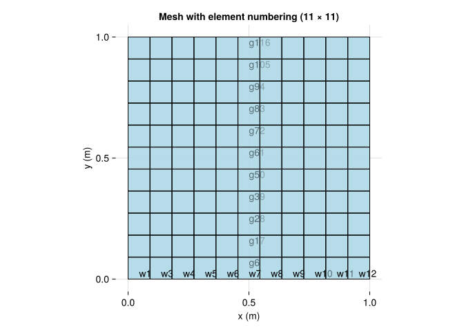
Volume elements are labelled gi and wall surfaces wi. These are the same indices used in the exchange factor matrix mesh.F_smooth and in the system matrices. Their rows and columns always start with the surfaces, followed by the volumes.

Step 2: Ray trace (with optional ray recording)

record_ids = [10, 20, 30]                          # optional: elements whose emitted rays are recorded for plotting
rec = RayRecorder(record_ids)                      # the ray recorder (also works in parallel)
mesh1(10^7; method = :exchange, rec = rec, verbose = false)   # ray tracing with the Sobol sampler
origins, endpoints = collect_rays(rec);            # the recorded rays, one line per ray

:exchange samples an absorption depth for every ray, and it is the tracer the ray recorder belongs to. :pathlength records each ray’s path through the medium instead and deposits along it, which makes it several times more accurate for participating media at the same ray count; it is the tracer used in Examples 3 and 4.

Step 3: Smooth

stats = smooth!(mesh1; verbose = false);           # enforce reciprocity and energy conservation on F_raw

smooth! produces mesh1.F_smooth and returns convergence diagnostics, one entry per spectral bin, so a run can be checked without reading the log:

all(stats.converged), maximum(stats.delta_smooth)  # did the projection converge, and the certified bound on the remaining reciprocity defect

(true, 3.0481274084910315e-15)

The named tuple also carries iteration counts (k_dykstra, k_ap, k_pcg_tot, k_pcg_max). See the smooth! docstring for the full description.

Step 4: Solve

solveEquilibrium!(mesh1, mesh1.F_smooth; verbose = false)   # solve the GERT system for the steady state

Step 5: Validate against Crosbie & Schrenker (1984)

The analytical solution for the dimensionless source function S(τ) = (T/T_hot)⁴ along the centreline of this problem is given by Crosbie & Schrenker (1984). Extracting the centreline temperatures from the solved mesh and comparing:

using Plots

# --- Top panel: solution temperature field via plotField ---
p1 = plotField(mesh1; field = :T, transparent_interfaces = true)
Plots.xlabel!(p1, "Position / m")
Plots.ylabel!(p1, "Position / m")
Plots.title!(p1, "Temperature distribution")

# Extract the centreline temperatures. The cells are stored row by row from the bottom (left to
# right within a row), so reshaping into an Ndim × Ndim matrix gives Tg_matrix[column, row].
all_temps  = [cell.T_g for cell in mesh1.fine_mesh[1]]     # gas temperature of every cell of the (single) coarse face
Tg_matrix  = reshape(all_temps, Ndim, Ndim)               # first index: column (x), second index: row (y)
centerline = Tg_matrix[div(Ndim + 1, 2), :]               # the middle column, from the hot wall upwards

# Dimensionless source function S = (T / T_hot)⁴ at the optical depth of every cell centre
S_computed  = (centerline ./ 1000.0) .^ 4                 # T_hot = 1000 K
tau_centers = range(1 / (2Ndim), 1 - 1 / (2Ndim), length = Ndim)   # τ = κ·y at the cell centres (κ = 1 m⁻¹, height 1 m)

# --- Crosbie & Schrenker (1984) analytical reference: optical depth from the hot wall, and S there ---
tau_ref = [0.0, 0.00611, 0.02037, 0.04251, 0.07216, 0.10884, 0.15194,
           0.20076, 0.25449, 0.31225, 0.37309, 0.43602, 0.50000, 0.56398,
           0.62691, 0.68775, 0.74551, 0.79924, 0.84806, 0.89116, 0.92784,
           0.95749, 0.97963, 0.99390, 1.00000]

S_ref  = [0.6293, 0.6198, 0.6017, 0.5767, 0.5460, 0.5108, 0.4724,
          0.4323, 0.3919, 0.3525, 0.3153, 0.2810, 0.2500, 0.2224,
          0.1981, 0.1768, 0.1584, 0.1424, 0.1287, 0.1171, 0.1073,
          0.0992, 0.0930, 0.0885, 0.0863]

# --- Bottom panel: centreline validation ---
p2 = Plots.plot(tau_ref, S_ref,
    linewidth = 2, color = :black, label = "Reference (C & S, 1984)",
    xlabel = "Optical depth τ",
    ylabel = "Dimensionless source function S(τ)",
    title = "Centreline validation",
    legend = :topright,
    guidefontsize = 12,
    tickfontsize = 10)

Plots.scatter!(p2, tau_centers, S_computed,
    color = :dodgerblue, markersize = 5, label = "RayTraceHeatTransfer.jl")
Plots.plot!(p2, top_margin = 8Plots.mm, bottom_margin = 8Plots.mm)

The top panel shows the 2D temperature field; the bottom panel compares the computed centreline source function (blue dots) with the analytical reference (black line).

To put a number on the agreement, the reference has to be evaluated in the same form as the solution. Each cell’s temperature follows from an energy balance over the whole cell, so the computed S is an average over the cell rather than a value at its centre. Next to the hot wall, where S is strongly curved, the two differ by more than the accuracy of the comparison, so the reference is averaged over each row of cells. ConvolutionInterpolations.jl interpolates the table with a high-order kernel (:b13 accepts nonuniform grids), and the midpoint rule on a fine subdivision gives the average over each row:

using ConvolutionInterpolations

S_ref_itp = convolution_interpolation(tau_ref, S_ref; kernel = :b13)       # the reference as a function of optical depth
tau_edges = range(0, 1, length = Ndim + 1)                                  # optical depth at the row boundaries (κ = 1 m⁻¹, height 1 m)

# Average of the reference over the row between optical depths a and b, by the midpoint rule
function row_average(a, b; n = 1000)
    width = (b - a) / n                                                     # width of one subinterval
    total = sum(S_ref_itp(a + (k - 0.5) * width) for k in 1:n)              # the reference at every subinterval midpoint
    return total / n                                                        # its mean over the row
end

S_ref_cells = [row_average(tau_edges[j], tau_edges[j+1]) for j in 1:Ndim]   # the reference averaged over each of the 11 rows

deviation = S_computed .- S_ref_cells                                       # solution minus reference, row by row
rms_dev   = sqrt(sum(abs2, deviation) / Ndim)                               # root-mean-square deviation along the centreline
max_dev   = maximum(abs.(deviation))                                        # largest deviation along the centreline

println("Deviation from Crosbie & Schrenker: rms = ", round(rms_dev; sigdigits = 2),
        ", max = ", round(max_dev; sigdigits = 2))                          # both in units of S, which runs from 0.09 to 0.63

Deviation from Crosbie & Schrenker: rms = 0.00051, max = 0.0012

For 10⁷ rays on the 11 × 11 mesh the rms deviation is 5.1 × 10⁻⁴ and the maximum 1.2 × 10⁻³, on a source function that runs from 0.09 to 0.63. It is largest in the first row above the hot wall, where the source function changes most steeply. At this number of rays the deviation comes mostly from the mesh, not from the rays: each cell carries a single temperature. Example 10 separates the two and shows the deviation shrinking at close to second order as the mesh is refined. The reference is tabulated to four decimals, so deviations below about 10⁻⁴ cannot be resolved by this comparison.

Step 6: Energy conservation, and why it is not the same as accuracy

After the solve, displaying the domain prints a summary whose last line is the relative energy conservation error: everything that leaves the elements, minus everything that is absorbed or reflected somewhere, relative to the total.

mesh1

RayTracingDomain2D
  geometry   1 coarse face → 121 volumes, 44 surfaces
  boundary   44 prescribed T, 121 prescribed source
  spectral   grey
  exchange   F_raw     165×165 sparse
             F_smooth  165×165 dense
  energy     6.34e-17 (relative conservation error)

The value is also available as mesh.energy_error. It sits at machine precision, and it does so for any number of rays: the rows of the exchange factor matrix sum to one, so the power that leaves the elements and the power that arrives at them are equal by construction, however well or badly the factors were sampled. Repeating the example with a thousand times fewer rays shows it, and shows at the same time that conservation says nothing about accuracy:

# rms deviation of the centreline source function from the row-averaged reference (as in Step 5)
function centreline_rms(m)
    all_temps  = [cell.T_g for cell in m.fine_mesh[1]]                  # gas temperature of every cell
    centerline = reshape(all_temps, Ndim, Ndim)[div(Ndim + 1, 2), :]    # the middle column, from the hot wall upwards
    S          = (centerline ./ 1000.0) .^ 4                            # dimensionless source function
    return sqrt(sum(abs2, S .- S_ref_cells) / Ndim)                     # rms deviation from the row-averaged reference
end

few = build_mesh(Ndim)                                   # the same domain again
few(10^4; method = :exchange, verbose = false)           # 10⁴ rays instead of 10⁷: about 60 per element
smooth!(few; verbose = false)                            # reciprocity on the noisy factors
solveEquilibrium!(few, few.F_smooth; verbose = false)    # solve with the smoothed factors
println("smoothed factors: energy error = ", few.energy_error, ", rms deviation = ", centreline_rms(few))

solveEquilibrium!(few, few.F_raw; verbose = false)       # solve again, now with the raw factors
println("raw factors:      energy error = ", few.energy_error, ", rms deviation = ", centreline_rms(few))

smoothed factors: energy error = 7.856564198231085e-17, rms deviation = 0.030991542252648656
raw factors:      energy error = 7.495556468289122e-16, rms deviation = 0.08083262797331256

rays	factors	energy conservation error	rms deviation from reference
10⁷	smoothed	6.3 × 10⁻¹⁷	5.1 × 10⁻⁴
10⁴	smoothed	7.9 × 10⁻¹⁷	3.1 × 10⁻²
10⁴	raw	7.5 × 10⁻¹⁶	8.1 × 10⁻²

Energy conservation is guaranteed by the formulation, so every GERT solution has it, the noisy ones included. How accurate a solution is, is a separate question: that depends on the number of rays, and it benefits from smoothing, which enforces reciprocity and here reduces the deviation by a factor of 2.6. A solution that conserves energy is therefore not automatically an accurate one, but an accurate GERT solution never has to be paid for with an energy imbalance.

References

Crosbie, A. L. & Schrenker, R. G. (1984). Radiative transfer in a two-dimensional rectangular medium exposed to diffuse radiation. Journal of Quantitative Spectroscopy and Radiative Transfer, 31(4), 339–372.

Bielefeld, N. M. (2026). A Radiation Exchange Factor Formulation with Proven Non-Negativity and Unconditional Energy Conservation. arXiv preprint, arXiv:2512.22157.